Vlookup Formula in Excel

Step by Step Vlookup Function in Excel

The VLOOKUP function is a premade function in Excel, which allows searches across columns. Using Vlookup fuction you can filter appropriate value from large amount of data based of give condition. Vlookup function is mainly used for two purpose, to find an exact match and to find the closest match. In other words Vlookup function retrieve data from a specific column in table.

In Vlookup V stands for vertical. It is typed =VLOOKUP and has the following parts:

Note: The column which holds the data used to lookup must always be to the left.

Note: The different parts of the function are separated by a symbol, like comma , or semicolon ;.

Importait point about Vlookup

• Vlookpu only loop Virtical
• Vlookpu only loop Right side

=VLOOKUP(lookup_value, table_array, col_index_num, [range_lookup])

• Lookup_value: This is the value you want to search for in the leftmost column of the table. It can be a number, text, or cell reference.
• Table_array: This is the range of cells that represents the table containing the data. It should include the column that contains the lookup value and the columns from which you want to retrieve the data.
• col_index: This is the column number within the table array from which you want to retrieve the data. For example, if you want to retrieve data from the second column of the table array, you would enter 2. The leftmost column of the table array is considered as column number 1.
• range_lookup: [optional] This argument determines whether you want an exact match or an approximate match. If you want an exact match, you can enter FALSE or 0. If you want an approximate match, you can enter TRUE or 1. If you omit this argument, Excel assumes an approximate match.

Step to Use Vlookup in Excel

• Select a cell (B2)
• Type =VLOOKUP
• Double click the VLOOKUP command
• Select the cell where search value will be entered (H3)
• Type (,)
• Mark table range (B2:G504)
• Type (,)
• Type the number of the column, counted from the left (2)
• Type True (1) or False (0) (1)
• Hit enter
• Enter a value in the cell selected for the Lookup_value F2(6)

Find an Exact Match Using Vlookup

In some cases we want exact match value

=VLOOKUP(H4,B5:E9,2,FALSE) // FALSE = exact match

Vlookup in Excel From Another Sheet

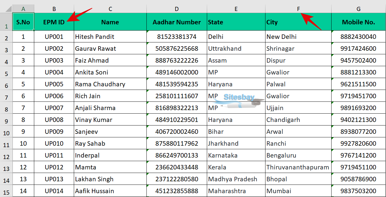
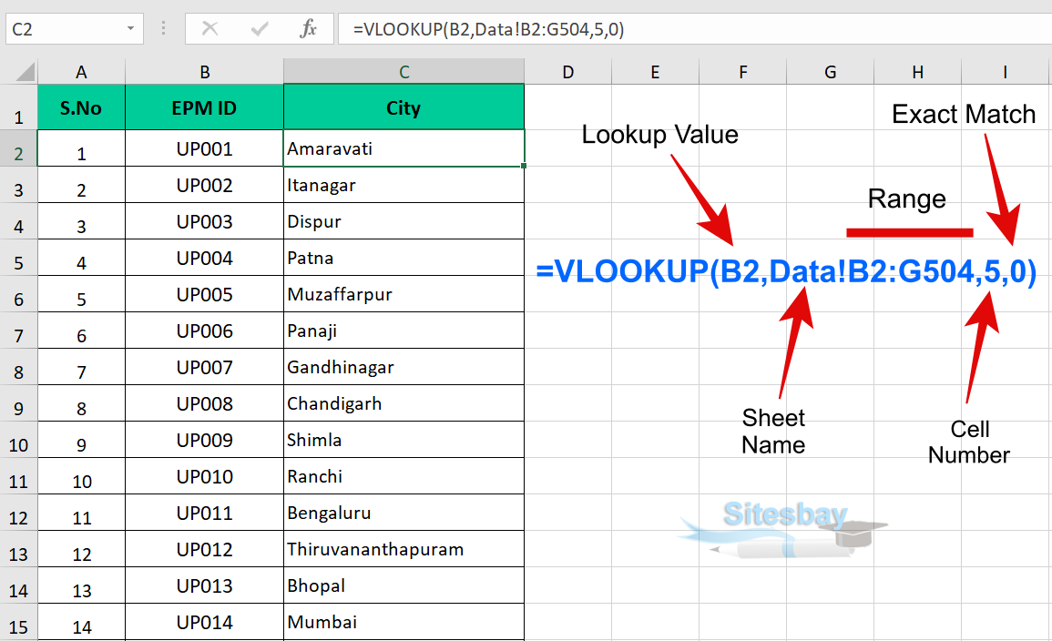
Here we Match Data based on EMP ID "From Cell B" and get City Column data form Other Sheet name Data. For Exact match use 0 or false.

=VLOOKUP(B2,Data!B2:G504,5,0)

Find an Closest Match Using Vlookup

=VLOOKUP(C5,$G$5:$H$10,2,TRUE) // TRUE = approximate match

There are certain limitations with using VLOOKUP—the VLOOKUP function can only look up a value from left to right. This means that the column containing the value you look up should always be located to the left of the column containing the return value.

Note: The Vlookup function can only look up a value from left to right.